Why fingerprint-MLP gradients don’t conflict, but graph-neural-net gradients do

Gradient-surgery methods (PCGrad, CAGrad, RCGrad, cosine-gating) promise to stop auxiliary tasks from dragging down a focal task in multi-task learning. Whether they do anything turns out to hinge on a choice you might think was orthogonal to it: the encoder. Swap a Morgan-fingerprint MLP for a message-passing graph net and the between-task gradient alignment — the one quantity every one of these methods acts on — jumps by an order of magnitude. This post is about why, and what that means for when to bother reaching for surgery at all.

This post records observations I made on multi-task learning while working on the OpenADMET PXR induction challenge — a research write-up of what I found, not a formal paper. I used Claude (Anthropic) for assistance with the writing and editing.

---

TL;DR

In multi-task learning with one focal endpoint and several auxiliary endpoints, the auxiliaries help or hurt the focal task through their gradients on the shared trunk. Whether gradient-surgery methods can do anything is decided by the cosine between the focal gradient and the auxiliary gradients — so the size of that cosine is the thing to understand.

The observation that started this: with a Morgan-fingerprint MLP that cosine is ≈0; swap in a graph encoder (D-MPNN) and it jumps ~10–20×. Only the graph encoder benefits from gradient surgery; for the MLP every combiner gives the identical result.

I built a probe to measure the cosine three ways — on the minibatches the optimizer actually sees, on the full training set, and on held-out data — at every epoch, per layer, from random initialization. Three findings:

1. The gap is real on the minibatch gradients the optimizer combines (~20×: GNN ~0.06 vs MLP ~0.003), and that is what decides whether surgery can help. The practical payoff is a clean double dissociation: averaging hurts the GNN and surgery recovers it, while the MLP is unaffected.
2. It is architectural, not about the input features. Feeding the same MLP a dense descriptor block instead of sparse fingerprint bits does not raise the operational cosine. At matched width, the graph encoder collapses the tasks into a lower-rank shared representation (effective rank 109 vs 155) with ~7× higher gradient overlap. And capacity modulates it — a narrow MLP develops the same entanglement — so it’s a continuum, not two species.
3. The alignment is a training-fit effect. It’s ≈0 at initialization and ≈0 on held-out data for every encoder; it is created during optimization, on the training distribution. (It is therefore not a measure of generalizable shared chemistry — but it still matters, because the optimizer acts on it; see §5c.)

Practitioner takeaway. Before reaching for a gradient-surgery method, measure the focal↔aux cosine on minibatches. ≈0 (a wide MLP on fingerprints, with any input) → every combiner collapses to averaging; surgery is a no-op and averaging is safe. Clearly positive (a graph encoder, or any capacity-starved shared trunk) → averaging can hurt and focal-aware surgery is worth trying. Don’t trust the raw small-batch number alone (noise biases it toward zero).

---

1. The hook: same data, same methods, opposite conclusions

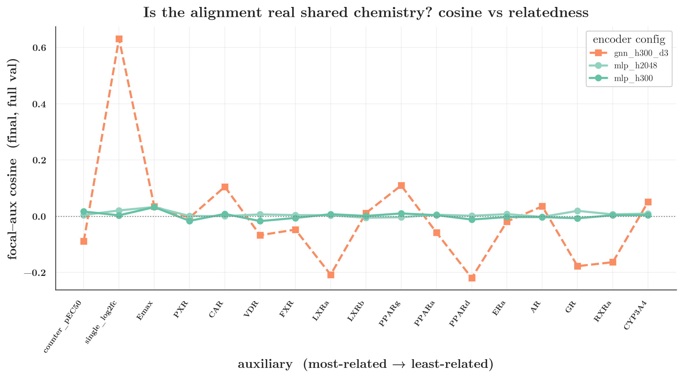
The focal task is PXR induction (pEC50 — a log-scale potency; higher = more potent), a nuclear-receptor endpoint with too little data to train a great single-task model — the canonical setup where you reach for auxiliary tasks. The auxiliaries are ordered by chemical relatedness, from same-compound assays and the closest NR1I receptors (PXR/CAR/VDR) out to mechanistically distant CYP3A4. Run the identical auxiliary-scaling sweep with two encoders, scored by RAE (relative absolute error; lower is better):

• Fingerprint MLP (Morgan ECFP → MLP trunk → per-task heads): every combiner — averaging, cosine-gating, PCGrad, CAGrad, RCGrad — gives the same focal error. A null result; the combiner you pick does not matter.
• D-MPNN (molecular graph → message passing → per-task heads): plain averaging suffers negative transfer as less-related auxiliaries pile on (focal RAE rises from 0.61 single-task to ~0.63), and focal-aware surgery recovers part of it.

Both encoders are trained end to end by the same loop; they differ only in what the shared trunk sees — a fixed Morgan fingerprint for the MLP, the raw molecular graph for the D-MPNN. (Neither is “the learned one”: the MLP’s trunk is learned too. And as §6 shows, it isn’t the input that drives the gap.)

The combiners being compared, one line each — they split along a single axis, whether the focal task is privileged over the auxiliaries:

• average (symmetric) — step along the unweighted mean of all task gradients. The plain-MTL baseline.
• PCGrad (Yu et al. 2020, symmetric) — for each conflicting pair of task gradients, project each out of the other’s direction, then average.
• CAGrad (Liu et al. 2021, symmetric) — step in the direction that helps the worst-off task most while staying close to the average gradient.
• cosine-gating (Du et al. 2018, focal-aware) — drop any auxiliary whose gradient points away from the focal gradient (negative cosine); average what remains.
• RCGrad (ours, focal-aware) — keep the focal gradient untouched and project each conflicting auxiliary onto the plane orthogonal to it, then average. An anchored variant of PCGrad — and not Dey & Ning’s (2024) learned-rotation RCGrad, which is a different method we don’t use here.

The symmetric methods treat focal and auxiliary tasks alike; the focal-aware ones protect the focal gradient. That distinction is the whole story below: when averaging hurts, it is the focal-aware methods that recover the loss — and on the MLP, where there is nothing to recover, all five collapse to the same answer.

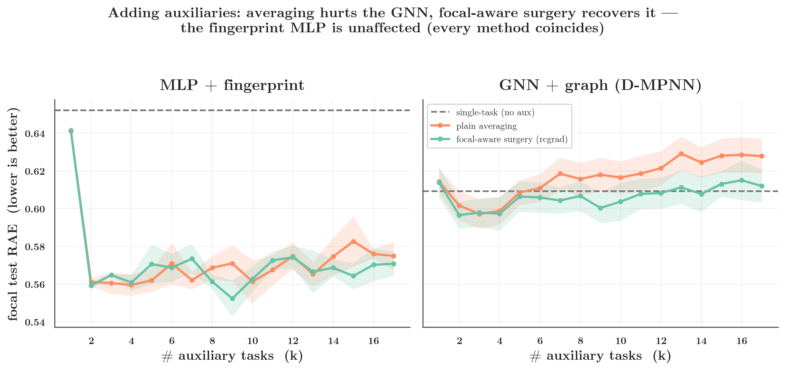
At the full auxiliary set (k=17): the MLP improves from single-task 0.652 → 0.575 with plain averaging and surgery adds nothing (0.571); the GNN worsens from 0.609 → 0.628 under averaging and surgery claws it back to 0.612. Two encoders, one dataset, one set of methods — opposite conclusions. It all traces to one number, so the number deserves scrutiny.

2. The data: focal task and auxiliaries

The focal task is the OpenADMET PXR induction endpoint. The auxiliaries are ordered by chemical/biological relatedness — same-compound assays first, then nuclear receptors from the closest subfamily (NR1I) outward to a mechanistically distant CYP enzyme. Every task is a single-output regression; molecules are featurized as Morgan ECFP bits (2048-d) by default (or ~200 dense RDKit 2-D descriptors in the input-decoupling experiment), and each task is split random 80/10/10 (train/val/test) with its own targets standardized on its own train fold. ChEMBL auxiliaries are de-duplicated against the PXR molecules to prevent leakage. The auxiliary-scaling sweep (§3) adds auxiliaries in the order listed below, so “k auxiliaries” = focal + the first k aux rows.

task	role	endpoint	N	train	val	test
pxr_pEC50	focal	PXR induction potency (pEC50)	4,139	3,311	413	415
pxr_counter_pEC50	internal aux	counter-assay / selectivity (pEC50)	2,647	2,117	264	266
pxr_single_log2fc	internal aux	21k single-conc. screen (log₂ FC)	21,003	16,802	2,100	2,101
pxr_Emax	internal aux	maximal effect (Emax), same compounds	4,139	3,311	413	415
chembl_PXR	aux · NR1I (closest)	PXR binding affinity (pChEMBL)	764	611	76	77
chembl_CAR	aux · NR1I	CAR binding affinity	204	163	20	21
chembl_VDR	aux · NR1I	VDR binding affinity	523	418	52	53
chembl_FXR	aux · NR1H	FXR binding affinity	3,264	2,611	326	327
chembl_LXRa	aux · NR1H	LXRα binding affinity	1,204	963	120	121
chembl_LXRb	aux · NR1H	LXRβ binding affinity	1,357	1,085	135	137
chembl_PPARg	aux · PPAR	PPARγ binding affinity	4,331	3,464	433	434
chembl_PPARa	aux · PPAR	PPARα binding affinity	2,836	2,268	283	285
chembl_PPARd	aux · PPAR	PPARδ binding affinity	1,865	1,492	186	187
chembl_ERa	aux · steroid/other	ERα binding affinity	4,470	3,576	447	447
chembl_AR	aux · steroid/other	AR binding affinity	2,952	2,361	295	296
chembl_GR	aux · steroid/other	GR binding affinity	3,043	2,434	304	305
chembl_RXRa	aux · steroid/other	RXRα binding affinity	1,390	1,112	139	139
chembl_CYP3A4	aux · CYP (farthest)	CYP3A4 binding affinity	5,576	4,460	557	559

So the focal endpoint has ~3.3k training molecules; the 17 auxiliaries span 204 (CAR) to 21k (single-concentration screen).

3. The observation: a 10–20× cosine gap

The number is the cosine between the focal task’s gradient and each auxiliary’s gradient, on the shared trunk (heads excluded), focal-centered, averaged over auxiliaries, averaged over training steps — the per-step (minibatch) focal↔aux cosine. Across experiments:

experiment (focal)	MLP + fingerprint	GNN + graph
auxiliary-scaling sweep (PXR)	0.007–0.011	0.05–0.18
diverse endpoint — Solubility (10k, TDC)	0.002–0.005	0.06–0.10

The second row is a fully independent check: TDC’s AqSolDB aqueous-solubility endpoint (~10k molecules) as the focal task, paired with six related ADME regression auxiliaries — lipophilicity, plasma-protein binding, Caco-2 permeability, volume of distribution, and hepatocyte and microsome clearance. Same ordering every time, and it holds across both endpoints (PXR and Solubility) and across graph architectures (D-MPNN, GINE). One subtlety worth stating up front: a slightly positive mean cosine does not mean “no conflict” — averaging is dragged down by the auxiliaries in the negative tail, and the mean is best read as a proxy for how strongly the tasks interact at all. The MLP’s ≈0 says the tasks barely interact through the trunk; the GNN’s ~0.06 says they interact a lot (some helpfully, some not).

But this is a minibatch, training-time number. A skeptic has three objections — and working through them is the whole story.

4. Three objections, one instrument

• Minibatch noise. A cosine estimated from noisy minibatch gradients is biased toward zero. How much of the MLP’s ≈0 is real orthogonality vs estimation noise?
• Parameter dimensionality. A wide MLP trunk has millions of parameters, and two gradients in a million dimensions are nearly orthogonal by default (concentration of measure). How much of the gap is just “the MLP trunk is bigger”?
• Training fit vs real signal. The cosine the optimizer sees is on training batches. Does the alignment reflect a stable shared structure, or just how the model fits the training set?

To answer all three I built one instrument and turned it on every epoch: a full-set, eval-mode, per-layer gradient-geometry probe. Every few epochs, in eval mode (dropout off), it computes each task’s shared-trunk gradient on the entire validation set and on the training set, and reports the focal-centered cosine overall and per layer, plus the gradient-norm ratio — including at epoch −1 (random init). (It’s measurement-only — a separate autograd pass that reads the gradients but never touches the optimizer, validated against a hand-computed cosine.) Full batch addresses the noise objection; per-layer + a parameter-count sweep addresses dimensionality; train-vs-held-out addresses the “real signal?” objection.

5. Controls: is the gap an artifact?

5a. Minibatch noise suppresses the observed cosine

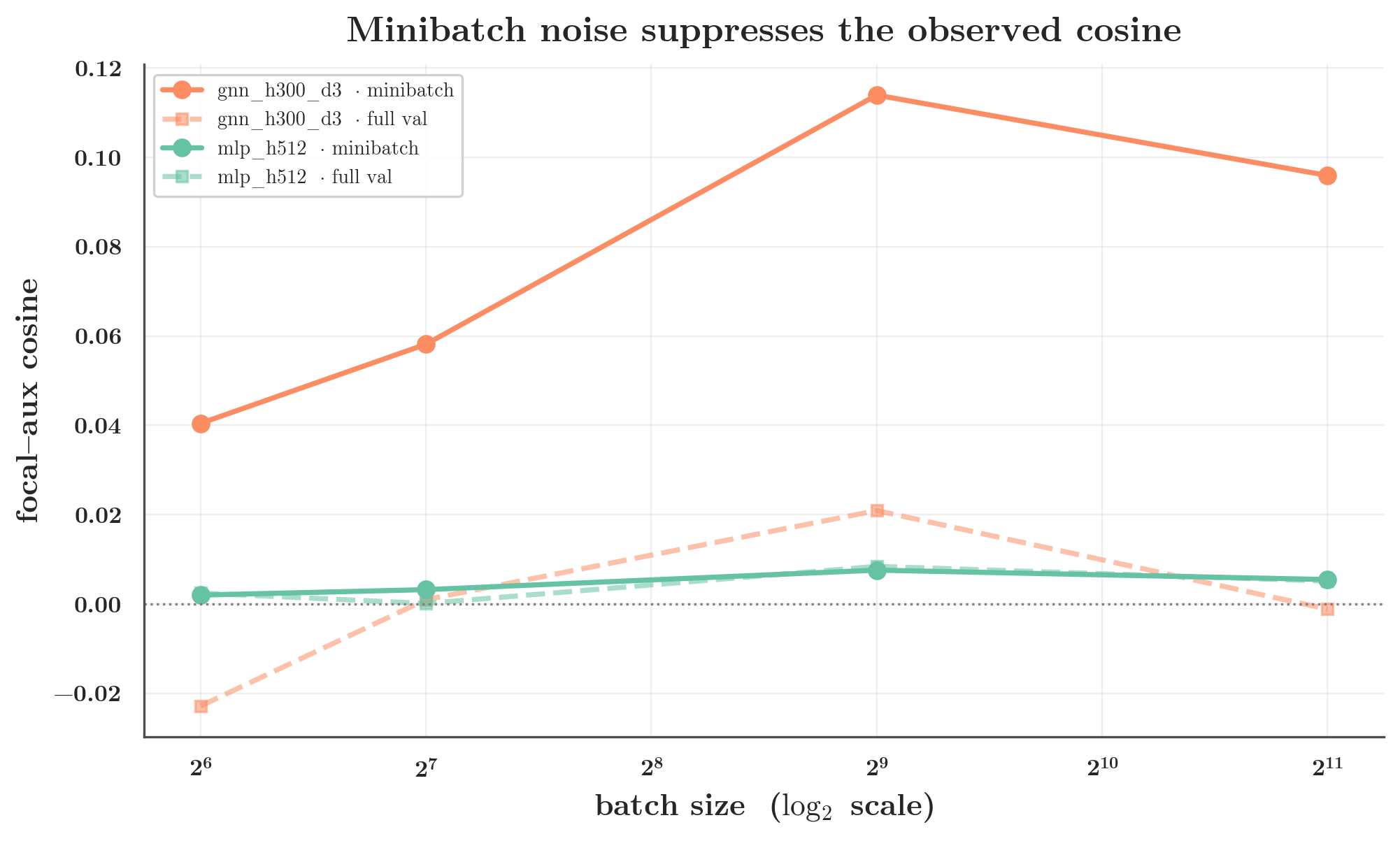
Sweeping batch size for a matched MLP and GNN (average):

batch size	GNN minibatch	GNN full-val	MLP minibatch	MLP full-val
64	0.040	−0.023	0.002	0.003
128	0.058	0.001	0.003	0.000
512	0.114	0.021	0.008	0.008
2048	0.096	−0.001	0.006	0.005

The GNN’s minibatch cosine more than doubles as the batch grows (0.04 → 0.11) — the small-batch number understates the training-distribution alignment because of noise. The MLP’s stays ≈0 throughout. So minibatch noise is real and shrinks observed cosines, but it does not invent the gap.

5b. Dimensionality explains much of the MLP-vs-GNN number — and reveals a continuum

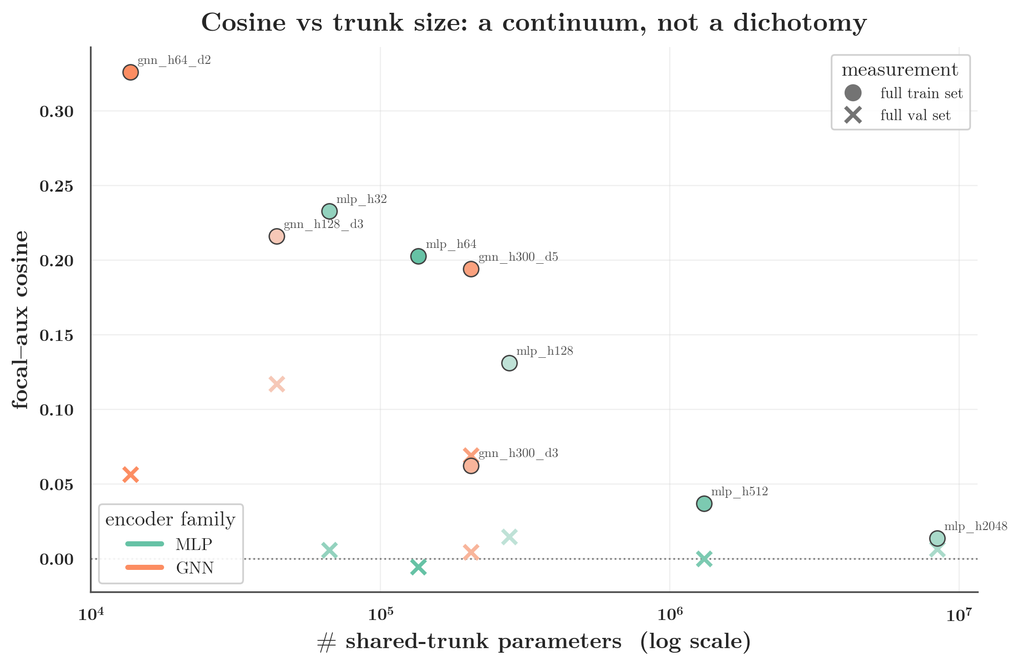
The entanglement sweep dials capacity while holding the task set fixed (the probe’s epoch-end cosines, mean over 3 seeds, random split). Configs are labelled by trunk width and depth — mlp_h2048 is an MLP with a 2048-unit hidden trunk, gnn_h300_d3 a depth-3 D-MPNN of width 300:

config	trunk params	minibatch	train (full)	val (full)
mlp_h2048	8.4M	0.002	0.014	0.007
mlp_h512	1.3M	0.003	0.037	0.000
mlp_h128	0.28M	0.004	0.131	0.015
mlp_h64	0.14M	0.004	0.203	−0.005
mlp_h32	0.067M	0.002	0.233	0.006
gnn_h64_d2	0.014M	0.045	0.326	0.057
gnn_h300_d3	0.21M	0.059	0.062	0.004
gnn_h300_d5	0.21M	0.086	0.194	0.069

Read the train column top to bottom: as the MLP narrows from 8.4M to 67K parameters, its full-batch train cosine climbs from 0.01 to 0.23 — into GNN territory. The wide MLP’s ≈0 is substantially its millions of parameters diluting the cosine; shrink the trunk and the entanglement appears. This is the single most important control: the gap is a continuum set by the effective dimensionality of the shared representation, not a dichotomy between architectures.

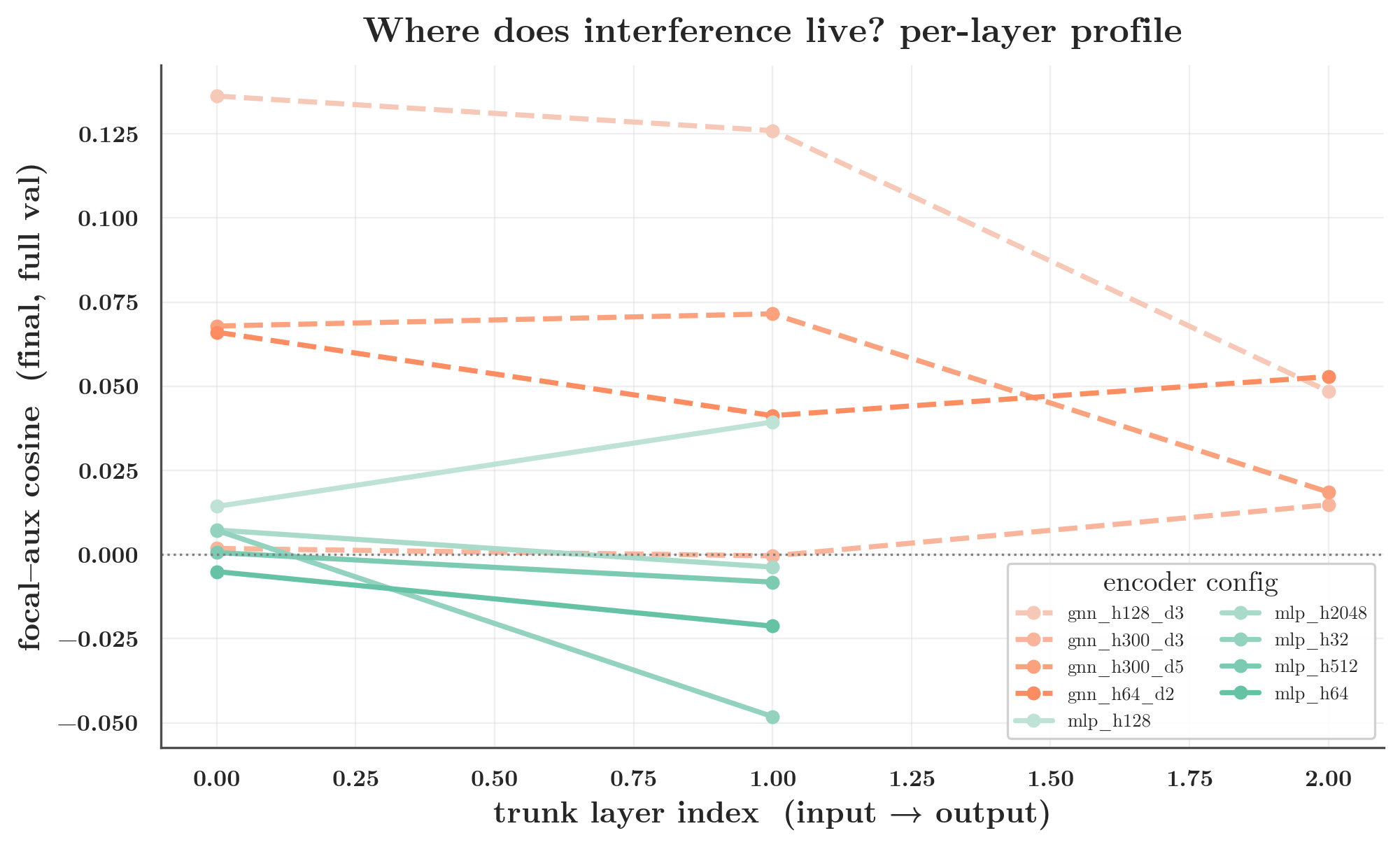
Where in the trunk does the (training-set) interference live? The per-layer profile concentrates it in the later, output-side shared layers — the wide early layer contributes the near-zero global value that the concatenated-trunk number reports.

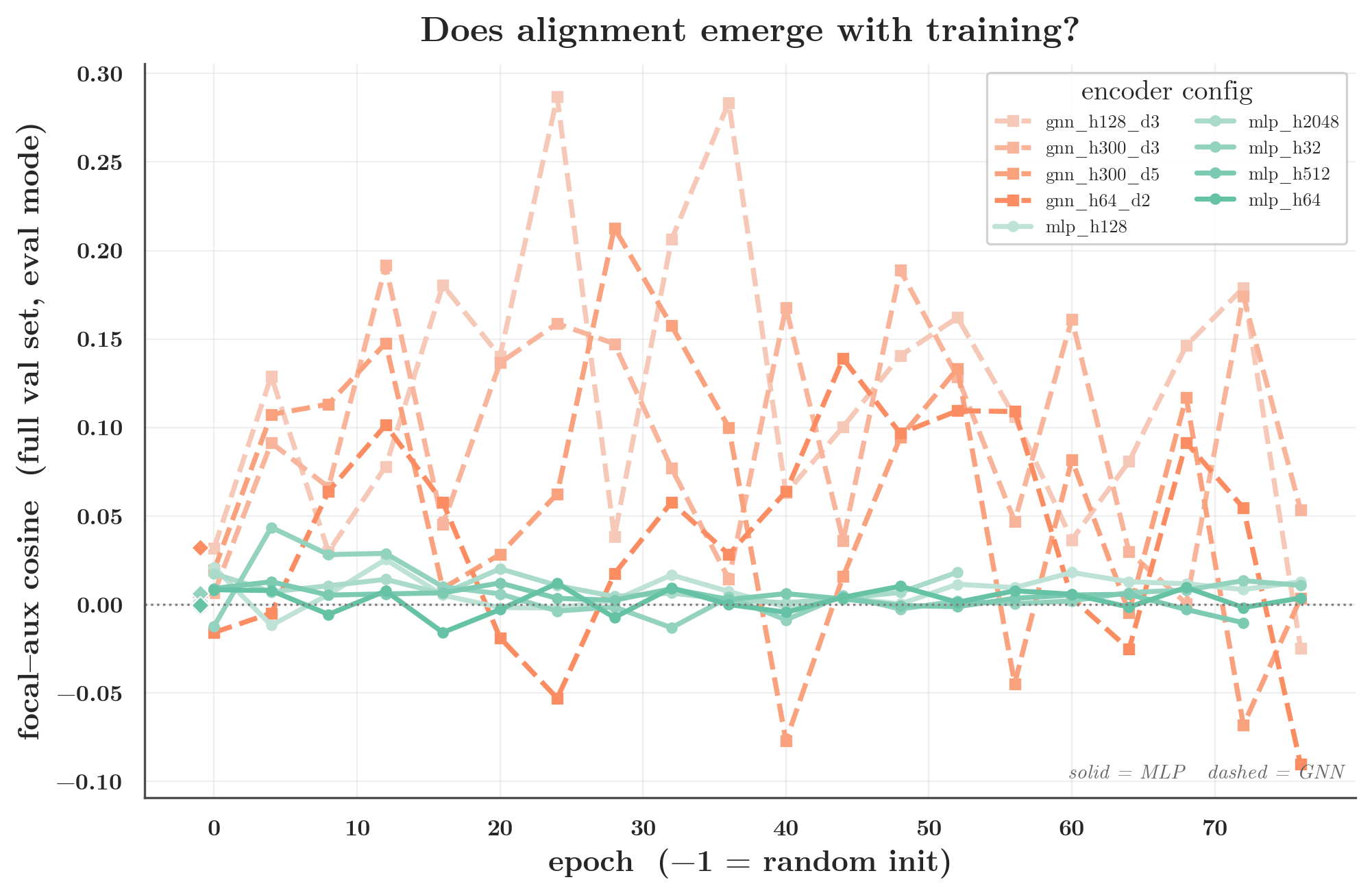
5c. The alignment is a training-fit effect, not a stable task property

Now read the val column above. It is ≈0 everywhere — for the narrow MLP (h32: train 0.23, val 0.006) and for the GNN (h300_d3: train 0.06, val 0.004). The earlier finding that a narrow MLP’s cosine “jumps to 0.13” was on the training set; on held-out molecules it is gone. The focal↔auxiliary gradient alignment is a property of how each model fits its training distribution, not a fixed signal the tasks carry. The per-epoch trajectory shows the same thing: every encoder starts at ≈0 at init, the train cosine grows with training, the held-out cosine stays near zero. Interference is created during optimization.

This does not make the conflict harmless. The optimizer averages minibatch gradients every single step, so when the focal and auxiliary minibatch gradients conflict, plain averaging drags the shared trunk away from the focal optimum — whether or not that conflict shows up as a held-out cosine. The held-out cosine being ≈0 only tells us the cosine is not a measure of shared generalizable chemistry; it does not say the training-time conflict is benign. The proof it isn’t benign is the headline figure in §1: averaging causes measurable negative transfer for the GNN, and focal-aware surgery recovers it. So the operationally relevant number is the minibatch cosine, and the gap there is exactly what tracks “does surgery help.”

6. Is it the input representation? (No.)

§5 established that the gap is real (not minibatch noise) and a continuum, not a clean architecture dichotomy. So what causes it? The natural causal hypothesis is that sparse, near-orthogonal ECFP bits let an MLP route tasks through disjoint inputs, while a denser or graph-derived representation forces them to share. I tested it directly — same MLP architecture, swap only the input: sparse ECFP vs ~200 dense RDKit descriptors (average, mean over seeds):

condition	minibatch	train (full)	val (full)
mlp_morgan (ECFP)	0.003	0.037	0.000
mlp_rdkit2d (dense)	0.002	0.133	0.006
mlp_morgan_h300	0.004	0.060	0.001
mlp_rdkit2d_h300	0.002	0.174	0.007
gnn_graph	0.058	−0.117	−0.070

A dense input does raise the MLP’s clean train cosine ~3–4× (0.04 → 0.13) — there’s something to the entanglement intuition at the representation level. But it leaves the minibatch cosine at ≈0.002 and the held-out cosine at ≈0. In other words: the input representation does not change the number the optimizer actually combines. Dense-vs-sparse input is not the operational cause.

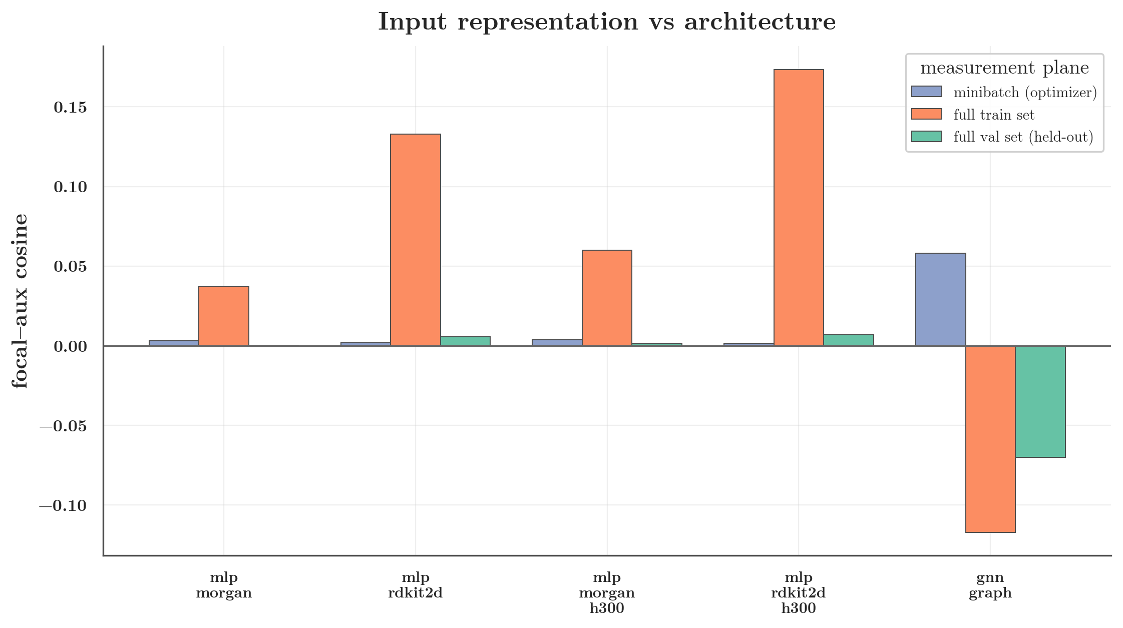
The decisive contrast is the bottom row: the graph encoder reaches minibatch 0.058 with the same auxiliary set on which the dense MLP sits at 0.002. Whatever the GNN is doing, an MLP fed a dense descriptor block does not reproduce it. (The GNN’s full-batch train/val cosine here is even slightly negative — a reminder that its alignment is a noisy, minibatch-scale, training-distribution effect, not a clean large-batch property; the operational claim rests on the minibatch number.)

7. The mechanism: a shared low-rank representation

If the input isn’t the cause, what is? The mechanism is in how each encoder organizes its learned shared representation. At matched hidden width (so representation dimension can’t confound), measuring the shared representation and the per-task gradients on the same data:

config	rep. effective rank	grad overlap (mean |cos|)	test RAE
mlp_h300	155 / 300	0.021	0.577
gnn_h300_d3	109 / 300	0.150	0.643
mlp_h2048	242 / 2048	0.016	0.560

Two quantities here, and they answer different questions. Effective rank (roughly, how many independent directions the representation actually spans) measures how compressed the shared representation is. Gradient overlap here is the unsigned, all-pairs mean |cos| among the task gradients — a measure of how much a set of tasks shares direction, distinct from the signed, focal-centered cosine used everywhere else in the post (which is why 0.150 is not in tension with the ~0.058 / ~0 signed numbers).

At the same width, the GNN packs the tasks into a lower-rank shared representation (109 vs 155) and its per-task gradients overlap ~7× more (0.150 vs 0.021). The MLP keeps a higher-rank, more task-disjoint representation in which gradients are nearly orthogonal. That is the mechanism behind the cosine gap: the graph encoder’s inductive bias is to share more of a smaller representation across tasks, so their gradients collide; the MLP spreads tasks out, so they don’t. Capacity modulates it (§5b): starve the MLP’s width and it, too, drops in rank and develops train-set entanglement.

8. The takeaway

• Gradient interference is created during training. It is near-zero at initialization and near-zero on held-out data for every encoder tested — but it is real on the minibatch gradients the optimizer combines, which is what determines the focal outcome.
• Its size is a continuum, governed by the effective dimensionality of the shared representation: a wide fingerprint MLP sits at the orthogonal extreme; a narrow MLP or a graph encoder collapses to a lower-rank, higher-overlap representation where gradients collide.
• It is architectural, not about dense-vs-sparse inputs. A dense descriptor block raises the clean train-set cosine but not the minibatch cosine the optimizer combines. The graph encoder’s representation-collapse is what produces operational interference.
• Whether gradient surgery can help is decided by the minibatch cosine. Measure it. ≈0 (a wide MLP, any input) → every combiner collapses to averaging; surgery is a no-op and averaging is safe. Clearly positive (a graph encoder, or a capacity-starved shared trunk) → averaging can hurt and focal-aware surgery is worth trying. Don’t trust the raw small-batch number alone — noise biases it down.

A closing note on the title. “Fingerprint-MLP gradients don’t conflict, graph-net gradients do” names the two ends of a spectrum, not two species. The real variable is representational entanglement — how much of a shared, low-rank representation the encoder forces the tasks through — and it is set by architecture and capacity together. A wide fingerprint MLP and a graph net are simply where two common defaults happen to land on that axis; narrow the MLP and it crosses over. The framing “MLPs and GNNs learn in fundamentally different regimes” is the wrong shape: it’s one axis, and what the axis governs is whether any gradient-alignment method has something to work with.

9. Methods

• Cosine definitions. All cosines are focal-centered (each auxiliary measured against the focal gradient) and use shared-trunk gradients only (per-task heads excluded). The minibatch cosine is taken in train mode (dropout active) and averaged over optimizer steps. The geometry probe instead uses the full split in eval mode, and records the overall cosine, a per-layer breakdown, and the focal/aux gradient-norm ratio — from epoch −1 (random init) onward, on both validation and train folds.
• The probe is measurement-only — a separate autograd pass that reads the gradients and never touches the optimizer state. Train-set probing is taken only at the endpoints (init/final) to keep it cheap; validation is probed every few epochs.
• Encoders. A fingerprint MLP (Morgan ECFP), a D-MPNN, and a GIN/GINE graph network. Featurizers: Morgan fingerprints (sparse bits) and RDKit 2-D descriptors (~200 dense physchem features, standardized on the train fold).
• Geometry metrics. Two underlie the §7 table. Effective rank (Roy & Vetterli 2007) measures how many independent directions the shared representation actually spans — i.e. how compressed it is. Gradient overlap is the unsigned, all-pairs mean |cos| among the per-task gradients (the quantity labelled “grad overlap” in §7), capturing how much a whole set of tasks shares gradient direction — as opposed to the signed, focal-centered cosine used everywhere else.
• Caveats. 3 seeds (10 for the GNN sweep); PXR focal, random split. The cosine is a trunk-gradient geometry measure; the RAE numbers are what tie it to focal performance. The GNN’s full-batch (vs minibatch) cosine is noisy and occasionally negative — another reason the operational claim rests on the minibatch measurement.

References

Gradient-surgery & multi-task optimization

• Du et al. (2018). Adapting Auxiliary Losses Using Gradient Similarity. arXiv:1812.02224. — the cosine-gating method.
• Yu et al. (2020). Gradient Surgery for Multi-Task Learning (PCGrad). NeurIPS. arXiv:2001.06782.
• Liu et al. (2021). Conflict-Averse Gradient Descent for Multi-task Learning (CAGrad). NeurIPS. arXiv:2110.14048.
• Dey & Ning (2024). RCGrad: rotating auxiliary gradients toward a target task for molecular property prediction. J. Cheminformatics 16:81. arXiv:2401.16299.
• Kendall, Gal & Cipolla (2018). Multi-Task Learning Using Uncertainty to Weigh Losses. CVPR. arXiv:1705.07115.
• Chen et al. (2018). GradNorm: Gradient Normalization for Adaptive Loss Balancing. ICML. arXiv:1711.02257.
• Kurin et al. (2022). In Defense of the Unitary Scalarization for Deep Multi-Task Learning. NeurIPS. — skeptic of gradient surgery.
• Xin et al. (2022). Do Current Multi-Task Optimization Methods in Deep Learning Even Help? NeurIPS. — skeptic.

Multi-task learning for molecular properties

• MTGL-ADMET: one-primary-multiple-auxiliary multi-task learning for ADMET. iScience (2023).
• AIM: adaptive interference-aware multi-task learning of molecular properties. arXiv:2509.25955 (2025).

Encoders & featurization

• Yang et al. (2019). Analyzing Learned Molecular Representations for Property Prediction (Chemprop / D-MPNN). J. Chem. Inf. Model. 59(8).
• Xu et al. (2019). How Powerful are Graph Neural Networks? (GIN). ICLR. arXiv:1810.00826.
• Hu et al. (2020). Strategies for Pre-training Graph Neural Networks (GINE). ICLR. arXiv:1905.12265.
• Rogers & Hahn (2010). Extended-Connectivity Fingerprints (ECFP/Morgan). J. Chem. Inf. Model. 50(5).
• Huang et al. (2021). Therapeutic Data Commons (TDC). NeurIPS Datasets & Benchmarks.

Analysis tools

• Roy & Vetterli (2007). The Effective Rank: A Measure of Effective Dimensionality. EUSIPCO. — the effective-rank measure used in §7.

Related representational-similarity tools (not reported in this post):

• Kornblith et al. (2019). Similarity of Neural Network Representations Revisited (CKA). ICML. arXiv:1905.00414.
• Weinberger et al. (2009). Feature Hashing for Large Scale Multitask Learning. ICML. arXiv:0902.2206.

Cite this post

If you found this useful, please cite it as:

Fooladi, H. (2026). Why fingerprint-MLP gradients don’t conflict, but graph-neural-net gradients do. https://hfooladi.github.io/posts/2026/06/why-fingerprint-mlp-gradients-dont-conflict/

@misc{fooladi2026gradalign,
  author       = {Hosein Fooladi},
  title        = {Why fingerprint-{MLP} gradients don't conflict, but graph-neural-net gradients do},
  year         = {2026},
  howpublished = {\url{https://hfooladi.github.io/posts/2026/06/why-fingerprint-mlp-gradients-dont-conflict/}},
  note         = {Blog post}
}