Research

One question runs through my work: how do you build a model that holds up on data it has never seen? I first met it in mechanistic models of developing cells, then in industry, predicting how cells respond to compounds and how proteins and degraders assemble, and now in my PhD on generalization in chemical space. The answer has less to do with architectures than with how you split the data, what you compare against, and whether you can tell in advance how far the new case is from the old ones.

The problem: drug discovery is extrapolation

University of Vienna · Kirchmair lab (Comp3D) · CD-Laboratory for Molecular Informatics in the Biosciences, with Boehringer Ingelheim and BASF

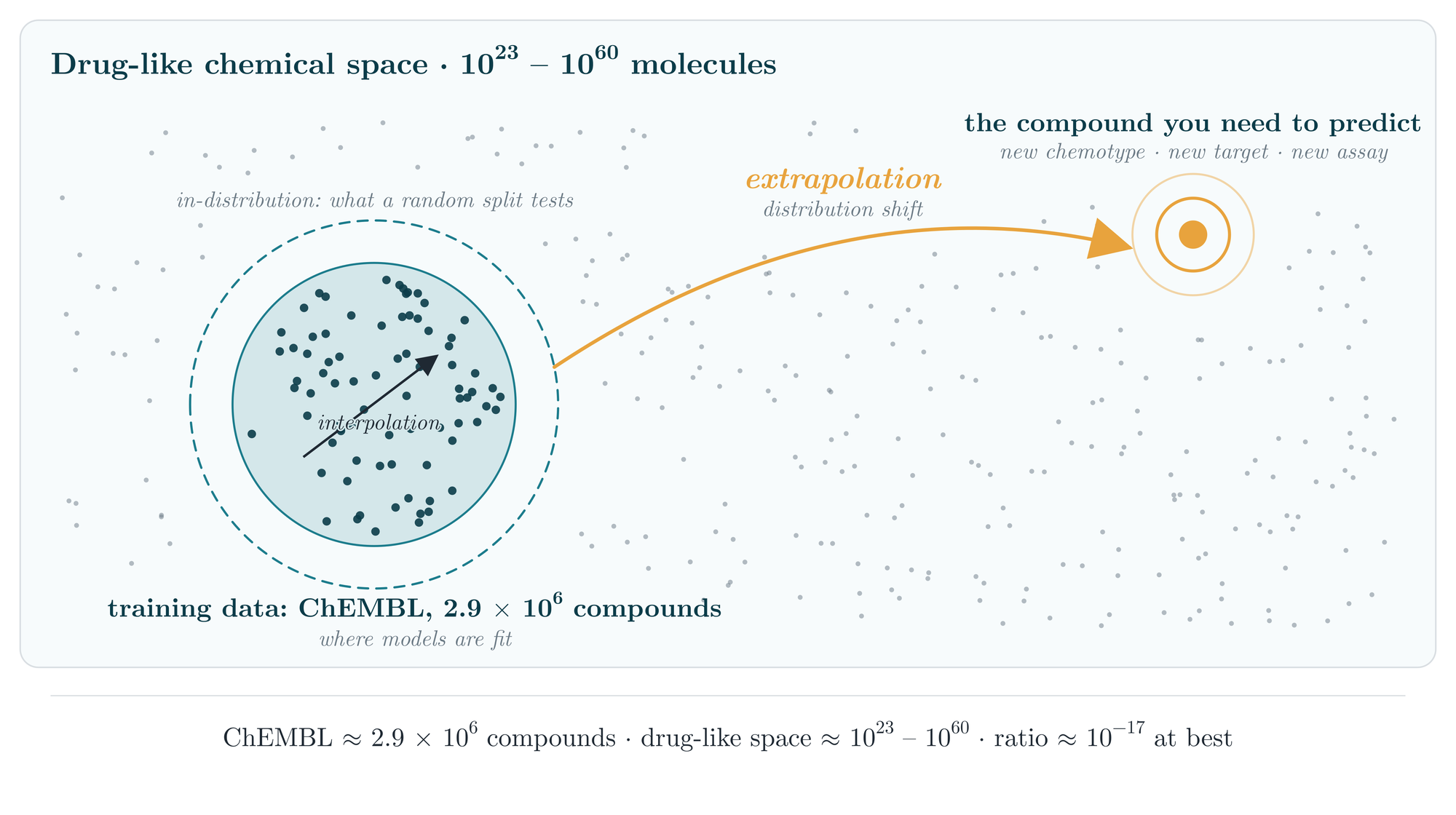
Drug-like chemical space is vast. Our data is not. ChEMBL holds bioactivities for roughly 2.9 million compounds, while the number of drug-like molecules is estimated at 10²³ to 10⁶⁰. Even against the smallest estimate, the measured fraction is about 10^-17. Any compound worth predicting, a new chemotype, a new target or a new assay, is therefore almost surely far from everything a model was trained on. A score on a random split only tells you how well the model interpolates among its neighbours; it says little about the leap that matters.

Where the data is and where the predictions are needed. Models are fit on the small, dense region of measured compounds; the compounds that matter lie far outside it. ML in drug discovery is, by definition, an extrapolation problem.

What the PhD does about it

Measure out-of-distribution honestly

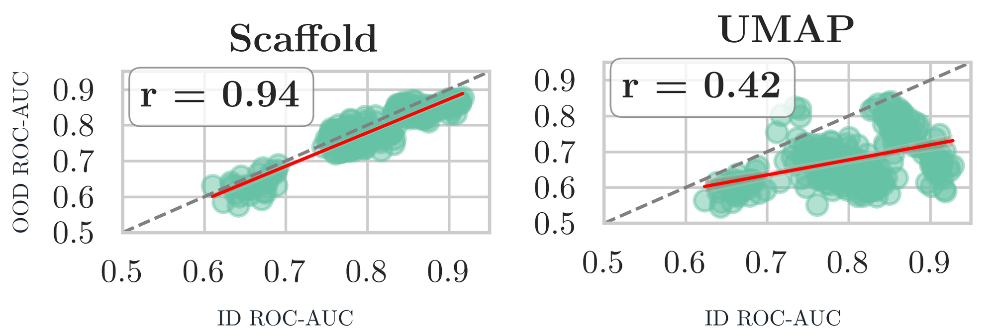
The first step is to define what “out of distribution” means for molecules and to measure how models actually behave there. We evaluated a broad set of models, from random forests to message-passing and pretrained graph neural networks, on bioactivity and ADMET datasets under many different splitting strategies. The result depends on the split far more than on the model. Scaffold splits, the community standard, are nearly as easy as random splits, and performance in distribution predicts performance out of distribution almost perfectly. Splits by chemical similarity clusters are the hard case: performance drops and the correlation collapses, so the model that looks best on in-distribution data is no longer a safe choice. Model selection is only trustworthy when the split mirrors the intended application.

In-distribution versus out-of-distribution performance for the same models and datasets under two splits. On scaffold splits (left) the two move together; on similarity-cluster splits (right) they barely do. From Fooladi et al., JCIM 2025; code and splitters in ALineMol.

Know how far a new task is from what you have

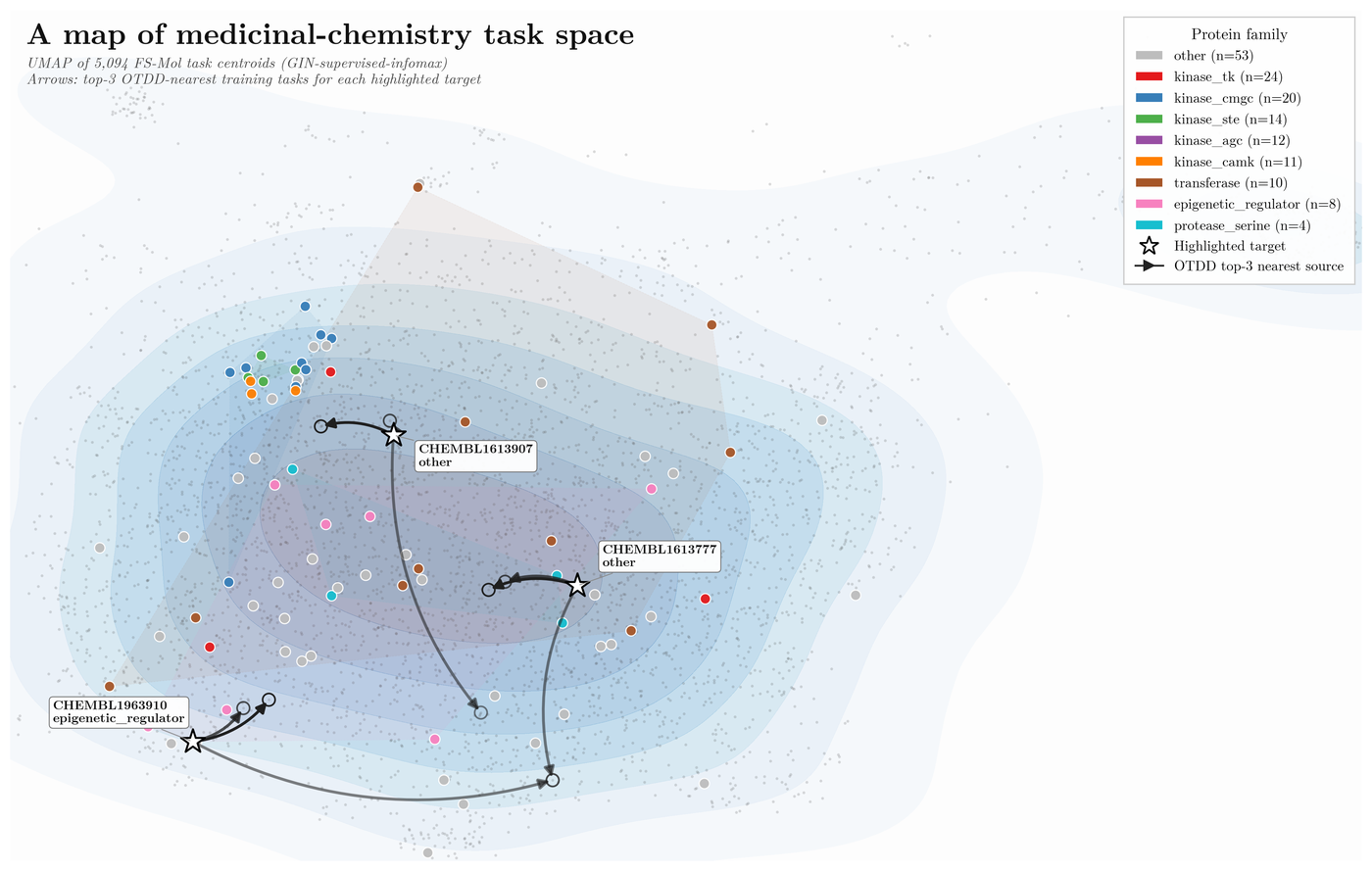
Most assays of interest have little data, so models borrow from related assays through transfer, multi-task or meta-learning. Whether that helps depends on how related the assays really are. We represent each bioactivity task by its chemistry and its protein target, measure its distance to every available training task with an optimal-transport dataset distance, and turn that into a hardness score. The score is computed before any training and it predicts the outcome: the harder a task by this measure, the smaller the gain from meta-learning. The same map tells you which source tasks are worth transferring from.

A map of medicinal-chemistry task space: FS-Mol bioactivity tasks coloured by protein family. Arrows point from three test tasks to their nearest training tasks under the optimal-transport distance. From Fooladi, Hirte and Kirchmair, JCIM 2024; the method is released as THEMAP.

Adapt at test time

Evaluation and task distance tell you when a model is about to extrapolate. The third part of the thesis, currently in preparation, is what to do at that moment: adapt the model to the region it is being asked about, using the unlabelled test molecules themselves, rather than hoping the training distribution was close enough.

Structure-based ML in industry

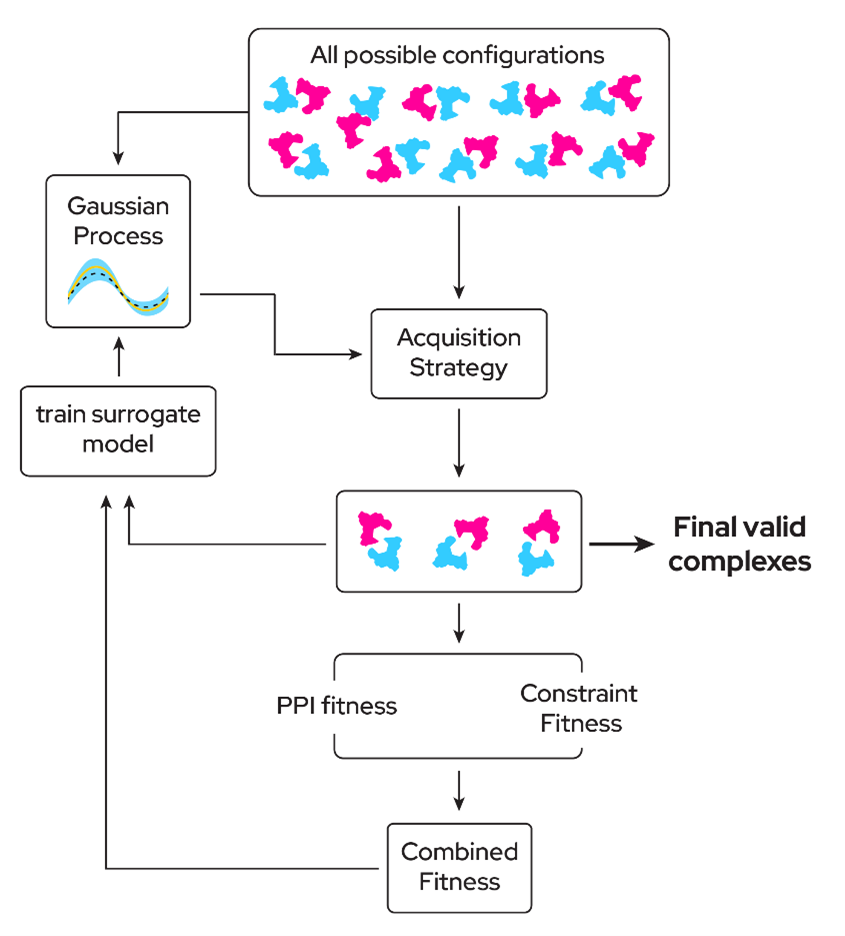
Before the PhD I led the machine learning team at Celeris Therapeutics in Graz, working on targeted protein degradation. The central modelling problem there is the ternary complex: a PROTAC molecule must hold a target protein and an E3 ligase together in a productive pose, and the number of candidate arrangements is enormous. BOTCP treats this as a Bayesian optimisation problem. A Gaussian-process surrogate and an acquisition strategy choose which configurations to evaluate, each is scored by a fitness that combines a protein-protein-interaction estimate with the PROTAC’s conformational constraints, and the result retrains the surrogate. On a benchmark of experimentally solved complexes the method recovers near-native poses within a small number of top-ranked clusters, at a cost of hours rather than days per complex. My part was the constrained conformer generation, the combined fitness and the cluster deployment; the method is published in Rao et al., AI in the Life Sciences 2023.

The BOTCP loop: sample ternary-complex configurations, score them with a combined protein-protein and constraint fitness, and let a Bayesian-optimisation surrogate decide what to sample next. Figure from Rao et al., 2023 (CC BY).

The same interest in making structure-based predictions trustworthy continued in Vienna. With Lan Vu we asked whether machine-learning pose sampling (DiffDock-L) can replace or complement classical docking in virtual screening, and found that the poses are only as useful as the scoring function that ranks them: rescoring with established physics-based functions is what turns a fast sampler into a usable screening tool (Vu, Fooladi and Kirchmair, JCIM 2025).

The path here

Mechanism first: stem-cell self-organization

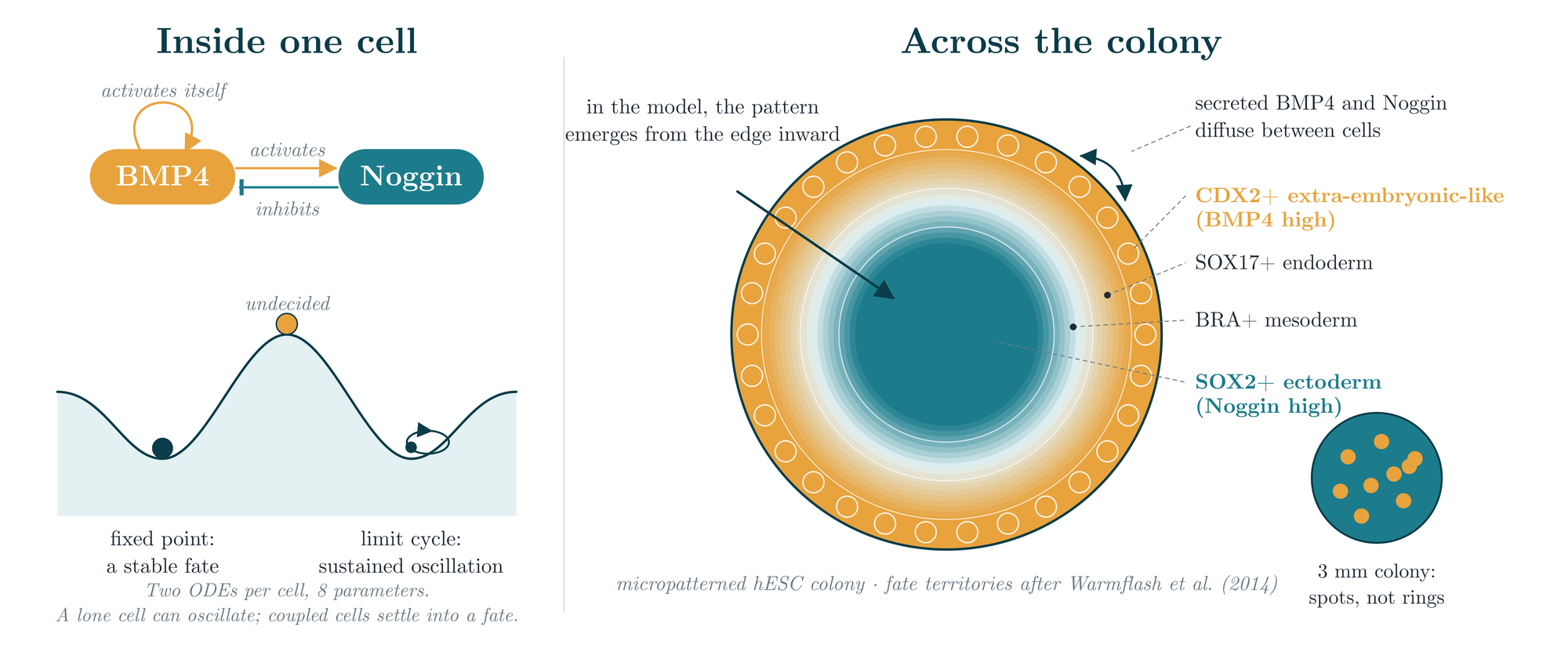
My master’s thesis at Sharif University asked how human embryonic stem cells on a micropattern organise themselves into concentric germ-layer territories with no external instruction. The answer that fit the experiments was small: every cell carries the same two-gene circuit, in which BMP4 activates itself and its inhibitor Noggin, both signals diffuse between neighbouring cells, and the pattern emerges from the colony edge inward. Two ODEs with eight parameters reproduce the rings, their response to colony size and culture conditions, and the spotted patterns seen in very large colonies. Published in Bioinformatics, 2019.

Inside one cell, a two-gene circuit; across the colony, diffusion between cells. Together they turn the Waddington landscape into a pattern-forming system.

Then the data arrived

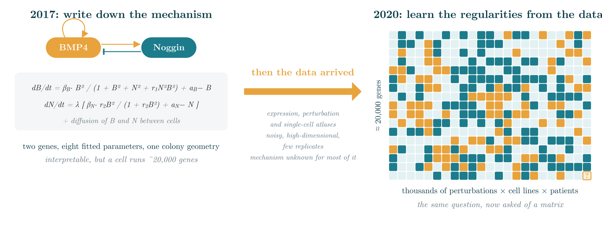
Two genes and eight fitted parameters explain a micropattern. They cannot absorb a perturbation screen, an expression atlas or a single-cell dataset, and for most of what those measure the mechanism is unknown. The question stayed the same, how does a cell decide what to become and how does it respond to a perturbation, but the tools had to change: at the Cambridge Systems Biology Centre I built my first models on expression data, autoencoders and cell-type classifiers, and then moved to learning the regularities of perturbation data directly.

From writing down the mechanism to learning it from data. The matrix on the right is the same biological question, now asked of about 20,000 genes at once.

Virtual cells: perturbation-response prediction

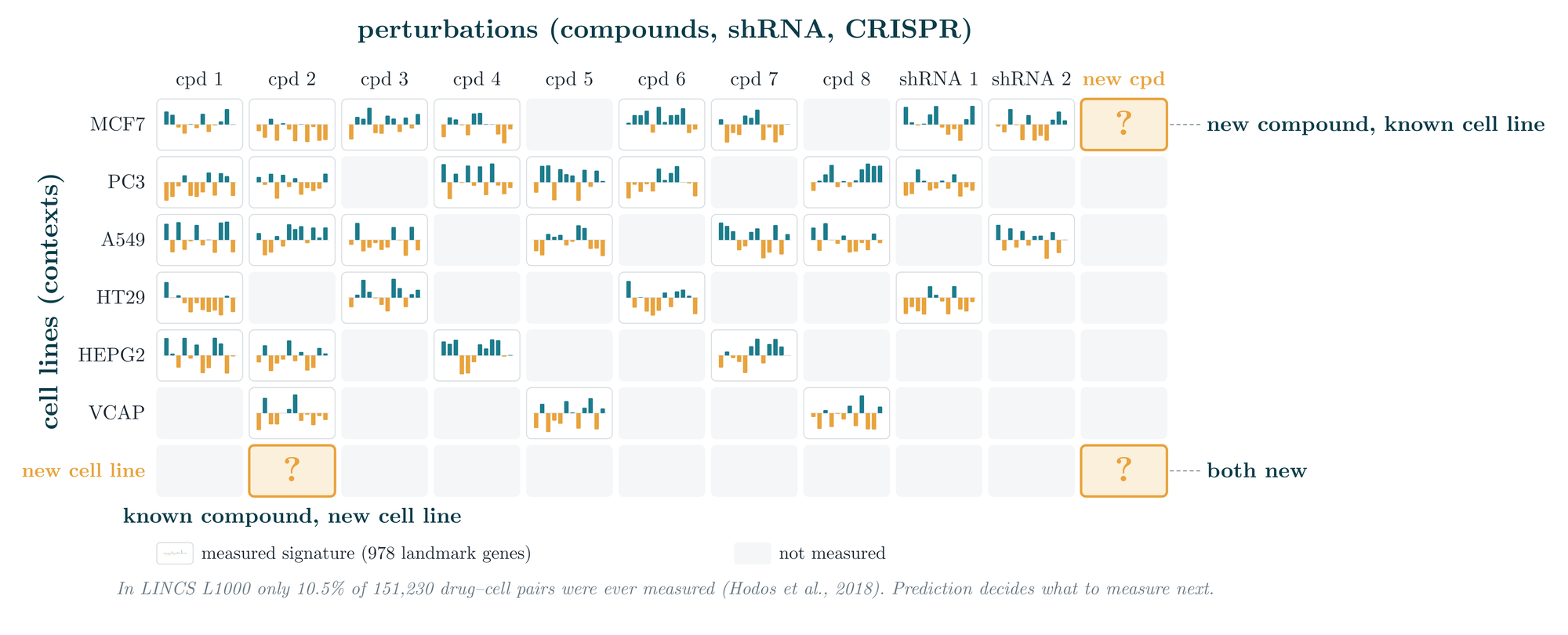
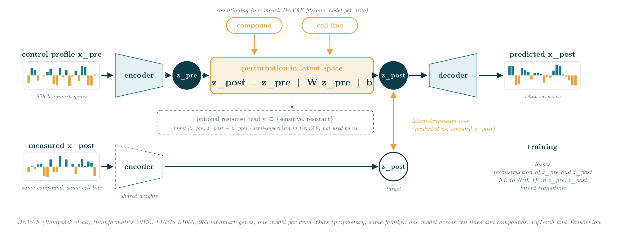
Between 2019 and 2020, at AI VIVO in Cambridge, I worked on “virtual cell” models: given a cell line and a small molecule, predict the change in the cell’s expression profile. The training data were the LINCS L1000 expression signatures. The core difficulty is sparsity: most compound and cell-line combinations were never measured, so a useful model has to extrapolate to new compounds, new cell lines, or both.

The perturbation matrix. Rows are cellular contexts, columns are perturbations, and a filled cell is a measured expression signature. In LINCS L1000 only about a tenth of the possible drug and cell-line pairs were ever measured (Hodos et al., 2018), which leaves three prediction settings of increasing difficulty: a new compound in a known cell line, a known compound in a new cell line, and both new.

The approach was a conditional variational autoencoder in the Dr.VAE family (Rampášek et al., 2019): encode the control expression profile into a smooth low-dimensional cell state, apply the perturbation as a learned displacement in that latent space conditioned on the compound and the cell line, and decode the predicted post-treatment profile. Training uses the measured post-treatment profile as the latent target, alongside the usual reconstruction and KL terms. Unlike the original Dr.VAE, which fits one model per drug, a single model is shared across compounds and cell lines.

A perturbation as a move in latent space. Top row, inference: encode the control profile, apply the learned perturbation in latent space, decode. Bottom row, training: the measured post-treatment profile, encoded with shared weights, provides the latent target for the transition loss.

What mattered most was evaluation. Dr.VAE’s own sanity check asks whether predicting the perturbation beats simply reconstructing the control profile; the effect is real but small and data-hungry, holding for well-covered drugs and not for thinly covered ones. The pipeline therefore shipped as a reproducible Nextflow workflow with explicit cold-compound and cold-cell-line splits and a training-mean baseline, and the data processing was released as lincs_processing. The same theme, that the split and the baseline decide what a model’s number means, runs through the out-of-distribution evaluation above.

Where this is going

My goal is to develop robust and trustworthy machine learning models for drug discovery. In practice that means putting the emphasis on rigorous evaluation: testing models under the distribution shifts they will actually meet, new chemotypes, new targets, new assays and new biological contexts, rather than on the convenient splits where every method looks good. A model earns trust when we know where it works, where it fails, and can tell the two apart before a prediction is used.

Selected publications

• 2025: Evaluating ML Models for Molecular Property Prediction on Out-of-Distribution Data (J. Chem. Inf. Model.)
• 2025: ML-Based Pose Sampling with Established Scoring Functions for Virtual Screening (J. Chem. Inf. Model.)
• 2024: Quantifying Task Hardness for Transfer Learning (J. Chem. Inf. Model.)
• 2023: Bayesian Optimization for Ternary Complex Prediction (AI in the Life Sciences)
• 2019: Enhanced Waddington Landscape Model with Cell-Cell Communication (Bioinformatics)

For the full list, see Publications · For talks and posters, see Talks